Deep Learning Introduction Part 1: Input Data and Neural Network Architecture

Posted on June 12th 2020.

This is part 1 of a blog series on deep learning. This series is intended as an introduction into deep learning, with an emphasis on the theory and the math that drives this technology. For this blog series we will be using Python 3 and Pandas. Also, some familiarity with linear algebra (vectors, matrices) will help. This first part will be about preprocessing example data, and outlines how a basic architecture of a feedforward neural network could look like. I hope you enjoy this series!

Introduction

A neural network is a computer algorithm composed of a network of artificial neurons. This network of aritificial neurons is able to learn patterns from example data, and is able to use this learned knowledge to perform some task. These artificial neurons are organised in layers. Deep learning is a popularized concept usually referred to when using a neural network with many layers to learn and perform some task.

Despite their consistent rise in popularity in recent years, neural networks and their fundamentall building blocks have been around for quite a while: Frank Rosenblatt laid out some of the fundational building blocks for the neural network in 1958. Thats over 60 years ago!

Over the years neural networks were improved, forgotten, improved, and forgotten again. For years neural networks couldn't do much, because, well, computers couldn't do much. In recent years however, with the help of the enormous rise of computing power, neural networks have proven to be invaluable in many many areas. With this technology becoming ever more usefull with each year, so does knowledge on how to build and train neural networks.

Input Data

The most important thing when working with neural networks is not the architecture of the neural network: Its the data. Why? You can build most complex neural network, but one rule always stays the same: Garbage in = Garbage out. So at the data we start!

Throughout this series we will build a neural network that is able to classify different types of shrubs based on their height and leave size. We will be using a generated dataset that is located here.

First we take a look at the data to see what we have:

import pandas as pd

df = pd.read_csv('shrub_dataset.csv')

df
"""
     Leave size (cm)  Shrub height (m)     Shrub species name
0           8.232398          3.064781            Hazel Shrub
1           6.374936          1.973804            Hazel Shrub
2           8.961280          3.854265            Hazel Shrub
3           8.242065          2.412739            Hazel Shrub
4           6.736104          2.559504            Hazel Shrub
...
...
97         4.047278          1.403136  Alder Buckthorn Shrub
98         5.911174          2.655614  Alder Buckthorn Shrub
99         4.131060          1.906048  Alder Buckthorn Shrub
"""

df.count()
"""
Leave size (cm)       100
Shrub height (m)      100
Shrub species name    100
"""

df['Shrub species name'].unique()

"""
array(['Hazel Shrub', 'Alder Buckthorn Shrub'],
      dtype=object)
"""

So our dataset has 100 rows, containing leave size and shrub height of two different shrub species. The task of the neural network will be to, given some shrub leave size, and some shrub height, to predict the shrub species. In this example the leave size and shrub height are the input features, and will be the neural networks input. The shrub species is what the neural network has to predict, and will be the neural networks output. In our example we will have 2 possible shrub species for the output: Hazel Shrub and Alder Buckthorn Shrub. So this means we will have 2 output classes. This task is a classification task, because given some input our neural network has to predict the output class. The fact that there are only 2 possible classes to predict makes this task a binary classification.

Note that for all these examples we already know the shrub species. Our goal was to make our neural network predict exactly this, so why do we look at data where we already know the answer? The reason for this is that our network first needs to learn how different leave sizes and different shrub heights can lead to different shrub species. Data such as this, in which we already know the class we want to predict is called labeled data. Data in which we do not know the class we want to predict is called unlabeled data. It is commonly hard to get alot of labeled data, because it often involes manual work to create. In our case the data is completely generated so luckily thats not the case here. However, suppose this was 'real' data, it means that expert on shrubs had a list of different leave sizes and shrub heights, and manually had to fill in the shrub species. It can take a while to get alot of labeled data that way.

Before we can use our dataset to train our network, there is some preprocessing we need to do. In itself the network can only convert numbers to numbers, so we will assign the number '0' to the Hazel Shrub and the number '1' to the Alder Buckthorn Shrub'.

For the input features, note that Leave size is in centimeters, and shrub height in meters. Another thing we will do is convert all these input values to 0 - 1 range. One of the reasons to do this is to prevent that a large feature (such as the shrub height in this case) has a disproportionate effect on the training. Here is the full preprocessing code:

import pandas as pd

df = pd.read_csv('shrub_dataset.csv')
# Extract the class column from the dataframe
# and conver the class names to numbers.
df_values = df.values
class_column = df_values[:, 2:3]
class_column[class_column == 'Hazel Shrub'] = 0
class_column[class_column == 'Alder Buckthorn Shrub'] = 1

# Drop the class column in the original df
df2 = df.drop(columns=['Shrub species name'])
# Normalise the features in the df
preprocessed_df=(df2-df2.min())/(df2.max()-df2.min())

# Insert the class column again
preprocessed_df.insert(2, 'Shrub species name', class_column)

preprocessed_df.columns=['leave_size', 'shrub_height', 'shrub_species']

# Write the preprocessed df to a csv
preprocessed_df.to_csv('preprocessed_shrub_dataset.csv')

The following is a visualisation of our preprocessed dataset:

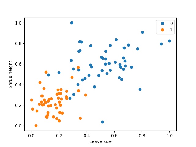
Figure 1: Visualisation of the preprocessed shrub dataset, with Hazel Shrub (0) in blue, and Alder Buckthorn Shrub (1) in orange.

Neural Network Architecture

In this example we will be looking at a type of neural network called a feedforward neural network. In a feedforward neural network the data flow is unidirectional: data comes in at the input, and goes out at the output.

The most fundamental building block of a neural network is the artificial neuron. The artificial neuron is a unit that takes input, does some mathematical transformation, and produces output. The mathematical transformation most commonly consists of multiplying an input vector by another vector, and adding a scalar. For example:

Where w is a vector containing weights, b is a scalar called the bias, x is a vector containing input values, and y is the scalar output. The weights and the bias are the learnable parameters of the neural network. Without them our neural network would not be able to learn anything. Recall that we want to classify different types of shrub species based on their leaf size and shrub height. The goal when training a neural network is to create a model that is most likely able to explain the observed data, using these learnable parameters of the neural network. When training, the values of the weights and the bias are adjusted slightly every iteration, in an attempt to find their optimal values. Usually before training the weight values are initialised at small random values, and the bias values are initialised at 0.

The artificial neurons are organised in layers. We will have 3 types of layers:

• The input layer. The input layer contains the input values without any weight or bias multiplication. In our case this is an input vector with 2 elements (shrub height and leave size).
• The output layer. The output layer is the final layer of our neural network, and outputs the predicted value. In our case this will be a single scalar in the 0 - 1 range, indicating the predicted shrub species.
• A hidden layer. Any layer that is not the input layer or the output layer is called a hidden layer. Their outputs are not directly observable. A hidden layer can contain any number of artificial neurons, and it is up to us to decide how many hidden layers there are, and how many artificial neurons they have.

We can chain these layers together. For this example, we will have the input layer, 3 artificial neurons in a first hidden layer, 3 artificial neurons in a second hidden layer and finally the output layer with 1 artificial neuron. From layer to layer, every artificial neuron is connected using weights. This means that with 2 input elements and 3 neurons in the first hidden layer we will have (2 x 3 ) 6 weights in between. From the first hidden layer to the second hidden layer, we will have 9 weights (3 times 3), and from the second hidden layer to the final layer we will have 3 weights (3 times 1). The number of bias units equals the number of neurons, so that means in total our neural network will have 25 parameters (6 weights + 9 weights + 3 weights + 7 bias units).

The following is a graphical representation of our neural network (excluding the bias units):

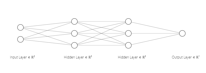
Fig1. Picture generated with help of http://alexlenail.me/NN-SVG/index.html

The following is a mathematical representation of the neural network until now:

With multiple neurons connected through multiple layers, the weights are aranged as matrixes. For example, the 6 weights in the between the input layer and the first hidden layer are arranged as a [2x3] matrix (2 input values, 3 neurons in the first hidden layer), and the bias here is a bias vector with 3 elements (because we have 3 neurons in the first hidden layer).

The depth of the neural network is the number of layers of the neural network. In our case the depth of the neural network is 3. This is because the input layer just represents the input data unmodified, as it is, without any weight and bias multiplication, and so it is commonly not counted when calculating the neural networks depth.

There is still an important ingredient missing from our neural network: an activation function. Suppose all that happened in a neural network with the data from input to output was multiplication of the input vector with some weight matrixes, and addition of bias some vectors. In this way, the neural network would only be able to learn a linear function.

This is where the activation function becomes very important. What the activation function does is introduce some kind of nonlinearity to the output. There are many different kinds of activation functions, but the most common being the Rectified Linear Unit (ReLU). ReLU is currently very popular for usage in the hidden layers because of its simplicity, while still being very powerfull. ReLU is easily implemented, and also easily differientable. ReLU is defined as:

The following is an implementation of ReLU:

def ReLU(input):
    if input < 0:
        return 0
    else:
        return input

So ReLU always outputs 0 when the input is negative, otherwise it outputs the unaltered input. We will use ReLU for the first hidden layer, and the second hidden layer.

For our output layer we will use the sigmoid activation function. The output of the sigmoid activation function stays within the 0-1 range. This is handy, because we can then assume that if the output is > 0.5, the neural network classified the input as a Hazel Shrub. Otherwise the neural network has classified the input as an Alder Blackthorn Shrub. The output of the sigmoid activation function saturates when the arguments are large or small. This activation function is defined by:

With the activation functions added, our neural network now looks like this:

Now that we have completed our neural network architecture, we can do a full example run through our neural network from input to predicted output. Some knowledge on matrix multiplication will be helpfull here. Take a look this page for a short tutorial on matrix multiplication.

For the input values, we will use the first row of our preprocessed dataset. The values (rounded to 2 decimals) for the leave size here and the shrub height here are 0.34 and 0.40. Because we do not have values for the weights and the bias, I will pick them here ourselves. As mentioned earlier, at the start of training the weights are commonly initialised as small random values, and the bias is 0. For now, for the weights I will pick random values between 0 and 2, and I will set all the bias values to -0.5. So:

Then:

And as a last step apply ReLU:

Now we can add this result as input to the second hidden layer. So:

And now we can use the result of the second hidden layer as input for the final layer:

And as a last step apply the sigmoid activation function:

So there we have it, we did a complete run from input to output through our network. This is also called a forward pass. However, when we look at the first row of our preprocessed dataset, we know that these input values we just used belong to a Hazel Shrub, to which we assigned to number 0. Given that our predicted output is 0.65, and higher than 0.5, it means our network predicted the shrub to be the Alder Blackthorn Shrub, to which we assigned the number 1. So thats completely wrong!

Howevever this is no problem. We haven't actually trained our neural network yet, and so all output values currently have no meaningfull relationship with the target shrub species at all. But how do you adjust the weight and the bias parameters, so that our neural network can predict the right shrub species? We need something that can tell us how wrong the predictions of the neural network are, and use this to update the values of our weight and bias parameters. This will be the topic for for the second part of this blog series.

Thanks for reading this blog! Like you, I am also learning, so if you see any errors in the text, or if anything is unclear to you, please let me know.